When interpreting Sentry pages, where information on known potential NEA impacts is posted, one must bear in mind that an Earth collision by a sizable NEA is a very low probability event. Objects normally appear on the Risk Page because their orbits can bring them close to the Earth’s orbit and the limited number of available observations do not yet allow their trajectories to be well-enough defined. In such cases, there may be a wide range of possible future paths that can be fit to the existing observations, sometimes including a few that can intersect the Earth.
Whenever a newly discovered NEA is posted on the Sentry Impact Risk Page, by far the most likely outcome is that the object will eventually be removed as new observations become available, the object’s orbit is improved, and its future motion is more tightly constrained. As a result, several new NEAs each month may be listed on the Sentry Impact Risk page, only to be removed shortly afterwards. This is a normal process, completely expected. The removal of an object from the Impact Risk page does not indicate that the object’s risk was evaluated mistakenly: the risk was real until additional observations showed that it was not. On the other hand, the impact Risk Page lists a number of lost objects that are, for all practical purposes, permanent residents of the Risk Page; their removal may depend upon a serendipitous rediscovery.
A summary of all known potential impacts is presented on the main Sentry page. The table quantifies the risk posed by the tabulated objects, using both the Torino Scale, which was designed primarily for public communication of impact risk, and the Palermo Scale, which was designed for technical comparisons of impact risk. A Palermo Scale value less than zero and, in most cases, a Torino Scale value of zero, indicate a risk below the so-called background level (more info here), which is the average risk from the entire NEO population. Typically, the risks posed by the potential impacts identified by Sentry are well below the background level, and hence, these events have been of academic or professional interest only, and not deserving of great public concern. Events with a Palermo Scale value greater than zero are very rare.
For each object listed on the main Risk Page there is a separate page providing more detailed technical information, some of which is included primarily to facilitate cross-checking among specialists involved in computing these predictions. The computation of Earth impact probabilities for near-Earth objects is a complex process requiring sophisticated mathematical techniques. An abbreviated and simplified explanation of the entire computation process is presented below and a Frequently Asked Questions page is available. For those who wish a more in depth mathematical explanation of this risk assessment process, please see the paper entitled Asteroid Close Approaches: Analysis and Potential Impact Detection by A. Milani, S.R. Chesley, P.W. Chodas, and G.B. Valsecchi (2002).
Every day, observations and orbit solutions for Near-Earth Asteroids (NEAs) are received from the Minor Planet Center (MPC) in Cambridge, Massachusetts. Once classified as an NEA, the asteroid is thereafter given automatic orbit updates within our Sentry system. A new orbit solution for an NEA is computed whenever new optical or radar observations for that object become available. Some high-priority objects are observed daily, while other objects go unobserved for days or weeks, even though they may still be bright enough to be seen. Optical observations cease when an object recedes from the Earth (becoming too faint to be seen even with moderate-size telescopes), or when the object moves into the daytime sky. Similarly, radar observations are possible only when the object is near enough to the Earth for the echo of a radar bounce to be detected. Once all the observations for an object have been collected, an orbit determination process is used to find the orbit that best fits all the observations.
The orbit is defined by six parameters (called the orbital elements) at an initial time (called the epoch). An object’s orbit is constrained to follow equations of motion that model the forces expected to be acting on that object at any given time. These forces are primarily the gravitational attraction of the Sun, the planets, the Moon, and 16 of the largest asteroids. Given the six orbital elements at the epoch, the object’s positions at other times are computed by a numerical integration, or propagation, of the equations of motion. In particular, the object’s position is computed at all the observation times, and given the position of the Earth and the observatory locations at those times, the expected values of the observations themselves are computed (e.g., the sky positions at the observation times). The difference between the computed value for the observation and the value actually measured by the observer is called the observation residual. The orbit for an object is determined using a process called differential correction that iteratively adjusts the six orbital elements until the sum of squares of all the observations residuals reaches a minimum value. The final result of the orbit determination process is called the best-fit or nominal solution. Note that the nominal orbit will not fit all the observations perfectly (i.e., the residuals will not all be zero), but it should fit all the observations to within their expected accuracies (typically less than 1 arc-second for optical observations). Also note that when new observations of the object become available, a new orbit solution must be determined in order to fit the augmented observation set.
It is important to understand that an object’s orbit is never known perfectly. Although the nominal orbit solution fits the observations best, slightly different orbits may still fit the observations to within their expected accuracies. There is in fact a whole set of orbits around the nominal that will fit the observations acceptably well: these all lie within what we call the uncertainty region about the nominal orbit. The ‘true’ orbit is expected to lie somewhere within this region. As new observations of the object are made, the uncertainty region becomes more tightly constrained and the range of possible values for the orbital elements narrows. As a result, objects that have been observed for decades will have highly constrained, well-known orbits, while newly discovered objects tracked for only a few days or weeks, will have relatively poorly constrained, uncertain orbits.
Once the nominal orbit and its associated uncertainty region have been determined, the object’s motion is numerically propagated forward in time for at least 100 years in order to determine its close approaches to the Earth. These nominal orbit close approach predictions are tabulated in our Earth Close Approach Tables along with other uncertainty-related information such as the minimum possible close approach distance, and the impact probability. The uncertainty-related parameters in the close approach tables are computed by propagating the uncertainty region from the epoch to the respective close approach times via so-called linearized techniques. Since these techniques lose accuracy when the uncertainties become large, we include only reasonably certain predictions in our Close Approach Tables. As a result, close approaches may be tabulated decades into the future for objects with well-known orbits, but only a few months or years into the future for objects with poorly known orbits. On the other hand, Sentry assesses the long-term possibilities of an Earth impact for all objects whose orbits can bring them close to the Earth, even those with poorly known orbits. To perform this risk analysis Sentry uses more sophisticated nonlinear methods.
Nonlinear analysis is required whenever the uncertainties in a close approach prediction are large. The position uncertainty of an asteroid is usually relatively small over the time span of the observations, but it usually grows, or stretches, as the object’s position is predicted farther and farther into the future. This uncertainty growth is especially fast along the track of the orbit. The evolution of uncertainties can be understood using the notion of so-called virtual asteroids (VAs). Suppose the uncertainty region around the nominal orbital solution is filled with a swarm of thousands or tens of thousands of virtual asteroids, each having slightly different orbital elements, but all fitting the observations acceptably well. Only one of these virtual asteroids is real, but we don’t know which one, although the central, nominal orbit is most likely to be the real one. The further a VA is from the nominal position within the swarm, the less likely it is to represent the real asteroid. If the three-dimensional positions of the VAs are plotted around the time of the observations, the swarm will take the shape of an elongated ellipsoid.
When the VAs are all numerically integrated forward in time, their slightly different positions in space allow each to undergo slightly different gravitational nudges (perturbations) from the planets and other perturbers. Over time, this swarm of virtual asteroids will spread out along the path of the nominal orbit, demonstrating how the uncertainty ellipsoid surrounding the asteroid’s nominal position evolves into a thin, elongated tube centered on the asteroid’s nominal orbit. Long-term orbital extrapolations can cause the asteroid’s position uncertainty tube to grow to great lengths, even extending one or more times around the asteroid’s entire orbit, and close planetary encounters can even cause the uncertainty region to fold and double back on itself. This type of numerical analysis, whereby many orbits are propagated forward in time to represent a single asteroid’s position uncertainty region, is the basis of the nonlinear techniques used by Sentry. The nonlinear impact-monitoring techniques used by Sentry are:
The conceptually easiest way to sample the orbital uncertainty is to generate a large number of virtual asteroids using a Monte Carlo technique. Millions of virtual asteroids must usually be propagated to characterize the region in parameter space leading to impacts with reasonable accuracy, making Monte Carlo simulation impractical for an automated impact monitoring system. To overcome this limitation, Sentry first runs a coarse Monte Carlo exploration with only 10,000 virtual asteroids to detect potential close approaches over the next 100 years. Then, starting from selected initial conditions, Sentry runs an extended orbit-determination filter that tries to converge to an impacting solution compatible with the observational data. The extended orbit-determination filter incorporates the impact condition as a pseudo-observation; in addition to minimizing the observation residuals, the extended filter minimizes the Earth miss-distance at the time of close approach. Suppose that the extended filter converges to an impactor. In that case, the output from the orbit-determination process includes the nominal impacting orbit plus a description of its uncertainty region. Finally, the impact probability is estimated using importance sampling to scale the uncertainty of the impacting orbit with the initial distribution of orbital uncertainty.
The parameter Sigma VI quantifies how well the impacting orbit fits the observations. Zero indicates the best-fitting, central (nominal) orbit and the further from zero, the less likely the event: for an orbit defined by six orbital parameters, roughly 83% of the uncertainty region is within 3-sigma.
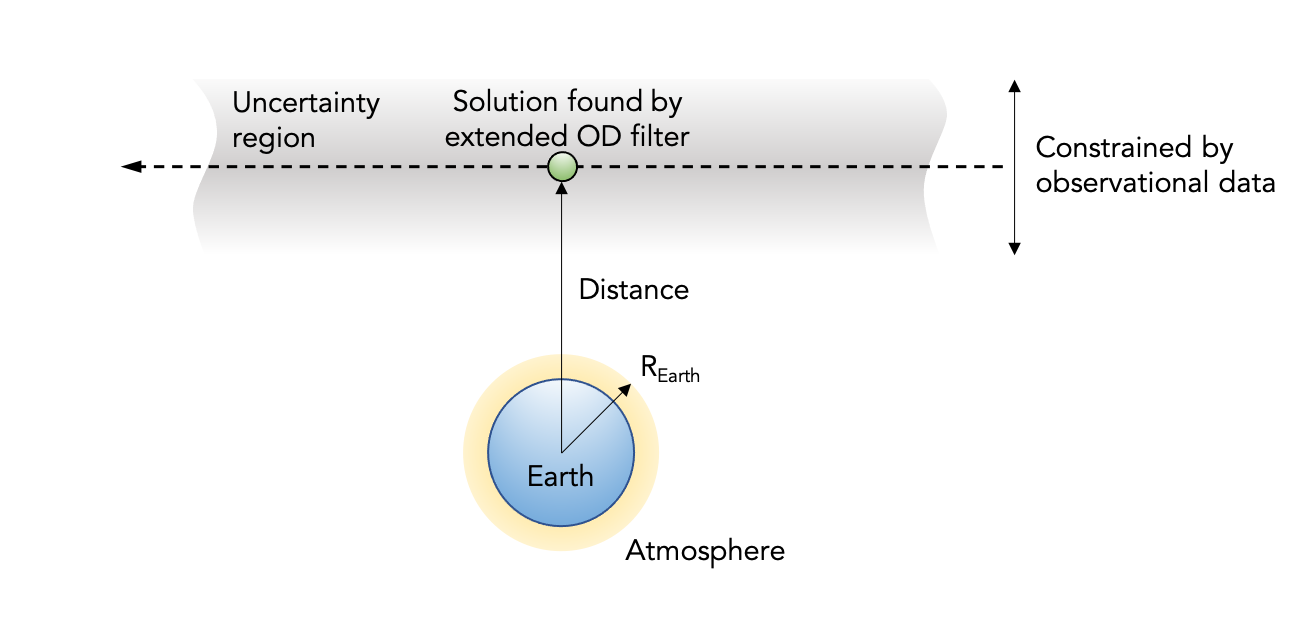
The impact probability analysis is based on the close-approach geometry on the B-plane, a plane defined as passing through the Earth’s center and being perpendicular to the incoming velocity vector of the NEA. The diagram below represents the B-plane and shows the point of closest approach found by the extended orbit-determination filter. This example corresponds to a near miss because the close-approach distance is greater than the Earth’s radius.
For more details about the impact pseudo-observation technique, refer to the paper entitled A novel approach to asteroid impact monitoring and hazard assessment by J. Roa, D. Farnocchia, and S.R. Chesley (2021).
The nonlinear analysis can be made computationally more efficient if only virtual asteroids along the central axis of the asteroid’s elongated uncertainty region are integrated forward in time. The assumption is then made that virtual asteroids along this “Line of Variations” (LOV) are representative of the nearby off-axis portions of the uncertainty region. The first step in the risk analysis is to numerically integrate the VAs on the LOV forward in time, and detect close approaches to the Earth. When a stream of consecutive VAs experience essentially the same close encounter, an automatic search is conducted to find the virtual asteroid that passes closest to the Earth. The motion of this particular virtual asteroid and its own local uncertainty region is then analyzed using linear techniques to determine if an impact is possible and, if so, to estimate the probability of impact. For pathological cases where an asteroid’s uncertainty region folds back on itself (due to a previous close planetary encounter) or where several complex streams of virtual asteroids are evident, a second form of nonlinear analysis may be undertaken. This technique, called Monte Carlo, samples the complete uncertainty region at epoch, not just the central axis, and uses a great many more virtual asteroids. Once again, all the VAs are integrated forward to the time of a close Earth approach, and monitored for possible impact. If, for example, a total of 100,000 virtual asteroids were integrated forward and two of these VAs manage to collide with the Earth in the year 2040 then the impact probability for the real asteroid in 2040 would be approximately 2/100,000, or 1/50,000.
As noted earlier, some of the entries on the individual object pages are meant to rapidly communicate and characterize the automatically generated results to colleagues for verification and, as such, they are not necessarily of general interest. Nevertheless, an effort is made here to clarify a few of the tabular entries on these pages. The particular circumstances of an Earth close approach are studied in the target plane, a plane defined as passing through the Earth’s center and being perpendicular to the incoming velocity vector of the NEA.
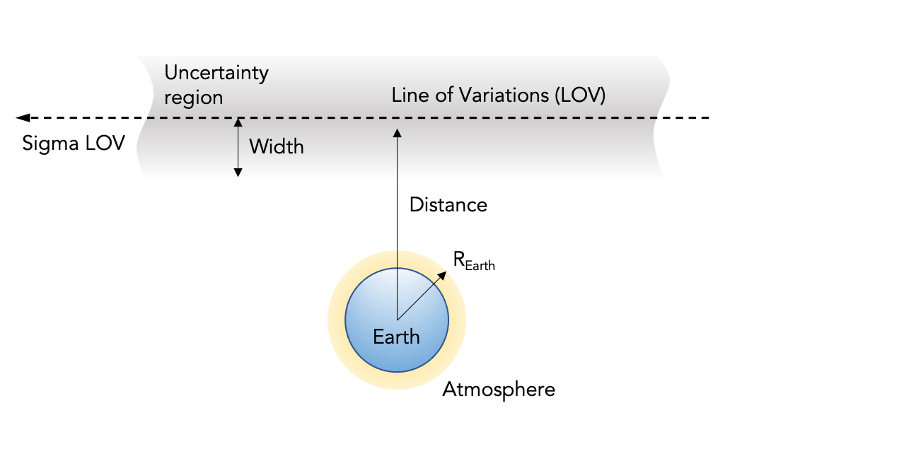
If we assume a particular asteroid’s position uncertainty region is a long three-dimensional tube stretched along its orbit, then a projection onto the target plane will reduce the uncertainty region to a two-dimensional strip centered on the Line of Variations and passing a certain Distance from the Earth’s center. If this Distance is less than 1 Earth radius then one of the virtual asteroids is known as a virtual impactor since it can strike the Earth. Sigma LOV is a measure of the deviation of the virtual impactor from the position of the central, or nominal, virtual asteroid. In other words, Sigma LOV is a measure of how well the impacting orbit fits the available observations. It is equal to zero for the best-fitting (nominal) orbit while orbits with values between -3 and +3 (“3-sigma”) comprise about 99% of the virtual asteroid swarm. The farther Sigma LOV is from zero, the less likely the collision with Earth. Since the intersection of the uncertainty region with the impact plane will form a narrow strip on the impact plane, three times the Width of this region in Earth radii will include more than 99% of the entire localized uncertainty region. Sigma Impact is computed from (Distance - R_Earth)/Width and it too is a measure of the impact likelihood. It has a value of zero when the LOV intersects the Earth and has increasing values as the central axis of the uncertainty region moves away from the Earth in the impact plane.